Basics of Stationarity and Unit root test
- Economics Major

- Oct 9, 2020
- 4 min read
Yes! we have come to this point now, where stationarity is highly important to further the research. So, stationarity is the basic assumption of many econometric models. Especially in case of forecasting. Stationarity in a time series model, says that all the moments of the data are constant and does not depend on time. By saying moments, I refer to the mean, variance, co-variance, autocorrelation structure and so on. If only all the moments of the data are constant it is called as strong stationarity, which is difficult to achieve. If only mean and variance are constant then it is called as weak stationarity. I also want to clear that 'white noise' is different from 'stationarity'. White noise is when the mean is zero and variance is constant. Thus, all white noise are stationary but not all stationarity are white noise. Then, researchers also get confused with 'random' and 'random walk'. We call the data as a random variable addressing the random probability or stochasticity of the data. However, random walk refers to non-stationarity, refering the random movement of data.
In the stochastic model, there are three kinds of non-stationarity: Random walk, random walk with drift and random walk with drift and trend.
i) Pure random walk is when the current year observation is equal to the last year observation and a random step up or down. Yt = Yt-1 + εt. This random step makes the data difficult to be predictable. Further, a random walk does not revert back to the mean after a shock.
ii) Random walk with drift refers to an addition of a constant term to the pure random walk. Yt = α + Yt-1 + εt. This constant is called as an intercept.
iii) Random walk with drift and trend is when the previous model also has a time variable in the equation which is trend. Yt = α + Yt-1 + βt + εt . This trend 't' here is a deterministic trend.
The presence of time series components such as trend, seasonality and irregularity, render the time series data non-stationary as it violates the assumption of non-dependancy on time. However, the presence of cyclicality does not cause non-stationarity. This is because the cyclicality does not follow a regular pattern or interval.
With this introduction, let's move on to stationarity tests.
Stationarity tests
Augmented Dickey Fuller test
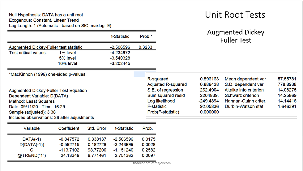
Augmented Dickey Fuller test is the widely known stationarity test. The test is used to check the serial correlation in the data. The basic Dickey Fuller test cannot take in more than one lagged variables which may lead to multicollinearity. But, Augmented Dickey Fuller Test (ADF), allows for more than one lagged variables. The lags are chosen based on the criterions such as Akaike Information Criterion (AIC), Hannan-Quinn Criterion, Schwarz Criterion and Bayesian Information Criterion (BIC). ADF test determines stochastic stationarity. The interpretation of ADF is test is based on the test statistics and p-value. The null hypothesis of ADF test is the presence of unit root in time series data. If the test (tau) statistics is higher than the critical values, the null hypothesis cannot be rejected. Looking at the results of ADF test below, we could conclude that the data is non-stationary with a stochastic trend. The stochastic trend can be removed by differencing.

Kwiatkowski–Phillips–Schmidt–Shin (KPSS) tests
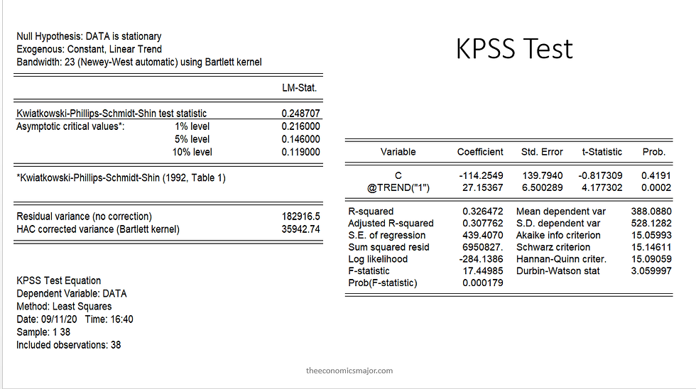
The speciality of KPSS test is to check the deterministic trend. This KPSS test is a Portmanteau test. The null hypothesis of KPSS test is stationarity of time series data. If the LM statistics is higher than the critical value, the null hypothesis is rejected and the series is non-stationary. The same data used in above ADF test was used in KPSS test also and was found that the data is non-stationary with a deterministic trend. The presence of deterministic trend must be removed before forecasting.

Apart from these tests, there are tests such as, Elliott–Rothenberg–Stock Test (P-test and DF-GLS test), Schmidt–Phillips Test (rho-test and tau-test), Phillips–Perron (PP) Test. It is advisable to use multiple tests before modelling for forecasting.
Kapetanios, G., A. Snell and Y. Shin (KSS) tests
All the test mentioned above are based on linearity assumption. Hence, to allow space for non-linear time series data, KSS test was designed in 2003. Even now, many tests are being designed to test stationarity. There is a seperate critical value table for KSS test which you can download here. The interpretation of KSS test is similar to ADF tests.
Zivot -Andrews tests
So we have tested for stationarity in a linear as well as non-linear assumption. What if the data has a structural break and we havent accounted for it in unit root tests. At times, the usual unit root tests doesnt behave well in a time series data with structural break. It may show a trend stationary data as non-stationary in the presence of structural break. Hence, we need to use unit root tests which account for structural break. Zivot-Andrews test allows for single breaks in the data while checking for unit root. There are other tests which are also famous and robust in case of Structural Break such as Narayan and Popp (with two structural breaks), Lee and Strazicich (with one and two structural breaks) and Enders and Lee Fourier tests.
HEGY unit root tests
Hylleberg, Engle, Granger and Yoo (1990) (HEGY) proposed a test for the determination of unit roots at each of the S seasonal frequencies individually, or collectively. This test is a seasonal unit root test. Seasonal unit root tests checks for stochastic seasonality in the data at regular frequencies. Other seasonal unit root tests are Smith and Taylor test, Canova-Hansen and Taylor unit root tests.
Apart from these tests, a simple correlogram also could help in finding stationarity. When the ACF dwindles slowly to zero then we could say that the data is non-stationary.


Comments